Seasonal Strength
seasonal_strength
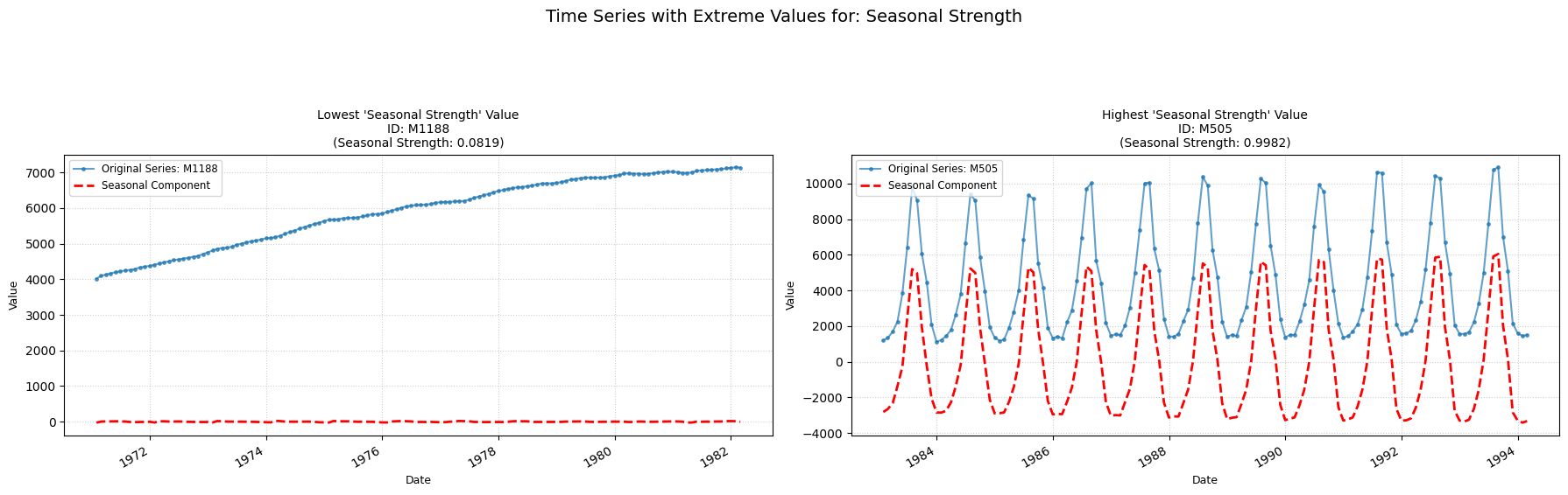
Computes the strength of seasonality within the time-series.
Low value: A value close to zero means there are few/none indicators of seasonality in the time series.
High value: A value close to one means there are strong signs of seasonality in the time-series.
Parameters Table
| Parameter | Type | Default | Description |
|---|---|---|---|
| period | int | 1 | Frequency of the time series (e.g. 12 for monthly) |
| seasonal | int | 7 | Length of the seasonal smoother (must be odd). |
| robust | bool | False | Flag for robust fitting. |
Calculation
-
STL Decomposition: The time series Yt is decomposed into trend (Tt), seasonal (St), and remainder (Rt) components, using an STL decomposition.
-
Detrended Series: The detrended series is calculated as Yt′=Yt−Tt=St+Rt.
-
Variances Calculation:
- The variance of the remainder component is calculated: Var(Rt).
- The variance of the detrended series is calculated: Var(Yt′).
-
Seasonal Strength Calculation: The value for seasonal strength is computed as max (0, 1 − Var(Yt′) * Var(Rt)). This value is capped between 0 and 1 and returned.
Practical Usefulness Examples
Retail Demand Planning: A high seasonal strength for ice cream sales (peaking in summer) allows a company to confidently plan production and marketing efforts around these predictable peaks and troughs.
Tourism Industry: Hotels can use the seasonal strength of booking data to optimize pricing, staffing and promotions, anticipating high and low seasons.